Weather Prediction with SVM, Decision Tree, and Gaussian

Weather prediction is a complex scientific process that involves analyzing various atmospheric conditions, historical data, and mathematical models to forecast future weather patterns. It plays a crucial role in our daily lives, aiding in planning activities, ensuring safety, and optimizing resource allocation. This time, we will try to forecasting weather using decision tree, svm and gaussian.

Before we jump into preprocessing, training testing and evaluating, we need to import the dataset and install scikit-learn matplotlib.

1. Import Dataset

!wget --no-check-certificate --content-disposition https://raw.githubusercontent.com/Shizu-ka/bruvv/main/weatherAUS.csv

2. Install scikit-learn

!pip install scikit-learn matplotlib

3. Import Necessary Library

import numpy as np
import pandas as pd
import seaborn as sns
import matplotlib.pyplot as plt
from collections import Counter
%matplotlib inline

# machine learning
from sklearn.linear_model import LogisticRegression, SGDClassifier, LinearRegression
from sklearn.tree import DecisionTreeClassifier
from sklearn.naive_bayes import GaussianNB
from sklearn.svm import SVC
from sklearn.neighbors import KNeighborsClassifier, KNeighborsRegressor

from sklearn import tree
from sklearn.preprocessing import StandardScaler
from sklearn.model_selection import train_test_split, GridSearchCV
from sklearn.pipeline import Pipeline
from sklearn.metrics import accuracy_score

4. Convert to Dataframe

ori = pd.read_csv('weatherAUS.csv')
df = pd.read_csv('weatherAUS.csv')
df_mean = pd.read_csv('weatherAUS.csv')
df.head()

5. Preprocessing

The next step is to do preprocessing. Keep in mind that you always welcome to do other method other than the one we do here. First we need to check how many null does every columns have.

df.isnull().mean()

Null Average

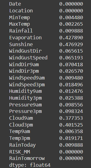
Because Evaporation, Sunshine, Cloud9am, Cloud3pm contain more than 30% zero values, they would be less helpful for the model so they were removed. Date is also not needed

df = df.drop(['Date','Evaporation','Sunshine','Cloud9am','Cloud3pm'], axis=1)
df_mean = df_mean.drop(['Date','Evaporation','Sunshine','Cloud9am','Cloud3pm'], axis=1)
df.head()

Machine learning model can not understand alphabets, so we need to convert it to number. The method is called features encoding.

Features encoding

cat_list = ['Location', 'WindGustDir', 'WindDir9am', 'WindDir3pm','RainToday', 'RainTomorrow']
for column in cat_list:
    df[column] = pd.Categorical(df[column])
    df[column] = df[column].cat.codes
    df[column].replace(-1, np.NaN, inplace=True)

    df_mean[column] = pd.Categorical(df_mean[column])
    df_mean[column] = df_mean[column].cat.codes
    df_mean[column].replace(-1, np.NaN, inplace=True)

The next step is to replace null value in the dataframe. Null value is a problem we will need to take care. If these null values are not handled properly, they can introduce biases or inaccuracies in the analysis and modeling process. There are many methods to fix this problem, such as

Mean/Median/Mode Imputation
Regression Imputation
Multiple Imputation
Hot-Deck Imputation
K-nearest neighbors (KNN)
MICE (Multivariate Imputation by Chained Equations)

In this experiment we will use KNN method, using KNNImputer from sklearn library.

from sklearn.impute import KNNImputer

def filling_null(feature, df=df):

    #make train set and test set
    temp_df = df.copy().drop('RainTomorrow', axis=1)
    df_list = list(temp_df.columns)
    df_list.remove(feature)
    temp_df.dropna(subset=df_list, inplace=True)
    train = temp_df.loc[temp_df.notna()[feature]]
    train_x = train.drop(feature, axis=1)
    train_y = train[feature]
    test = temp_df[temp_df.isnull()[feature]].drop(feature,axis=1)

    #run machine learning model and predict null values
    KNN = KNeighborsRegressor(n_jobs=-1)
    KNN.fit(train_x, train_y)
    change_NaN = KNN.predict(test)
    index_list = test.index.tolist()
    for i in range(len(change_NaN)):
        df.at[index_list[i], feature]= change_NaN[i]

    #return dataset which had been changed
    return df

Apply imputer

apply_list =['MinTemp', 'MaxTemp', 'WindGustDir', 'WindDir9am', 'WindDir3pm', 'Humidity9am',
             'Humidity3pm', 'Pressure9am', 'Pressure3pm']
for feature in apply_list:
    df = filling_null(feature = feature)

Check if there is any null value left

print(df.isnull().values.any())
print(df_mean.isnull().values.any())

True
True

True means there are still null values left in both dataframe. Why is this happening? The reason is the KNN imputation method relies on finding the nearest neighbors based on the available features to impute the missing values. However, if there are no similar data points with non-null values for some feature, the imputation may not be successful.

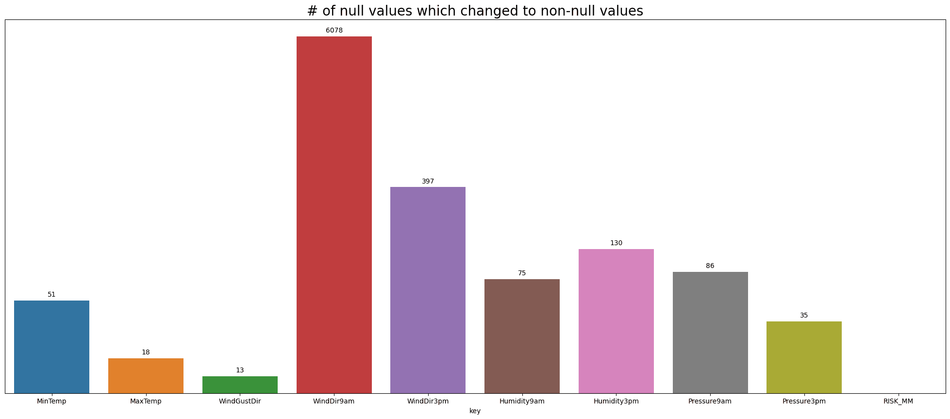
As an extension, we can see how many null value changes per features. Sometimes too many changes means we manipulating the dataset. Because imputer is not always right at predicting true value.

Visualization of null changes

#getting information of number of null variable changed
df_columns = list(df.columns)
changed_dict = {}
for col in df_columns:
    changed_dict["%s" %col] = len(df[col].dropna()) - len(ori[col].dropna())

#delet features which did not changed at all
pop_list = ['Location','Rainfall','WindGustSpeed','WindSpeed9am','WindSpeed3pm','Temp9am','Temp3pm','RainToday','RainTomorrow']
for feature in pop_list:
    changed_dict.pop(feature)

#make list of key and value to visualize the graph
key_list = []
value_list = []
for key, value in changed_dict.items():
    key_list.append(key)
    value_list.append(value)

temp_df = pd.DataFrame()
temp_df['key'] = key_list
temp_df['value'] = value_list

#visualization
plt.figure(figsize=(25, 10))
plot = sns.barplot(x='key',y='value', data=temp_df)
for p in plot.patches:
    plot.annotate(format(p.get_height(), '0.0f'),
                   (p.get_x() + p.get_width() / 2., p.get_height()),
                   ha = 'center', va = 'center',
                   xytext = (0, 9),
                   textcoords = 'offset points')
plt.yscale('log')
plot.axes.get_yaxis().set_visible(False)
plt.title('# of null values which changed to non-null values', fontsize=20)
plt.show()

Changes of null value

Now from the previous experiment, we still have rows with null values. Now to fix this we can just use mean to replace those null value.

df_Xnul = df.fillna(df.mean())
print(df_Xnul.isnull().values.any())

False

Now our preprocessing is finished.

6. Split Data Train & Test

The target class in this experriment is, wether its rain tomorrow or not.

X = df_Xnul.drop(['RainTomorrow'], axis=1)
y = df_Xnul['RainTomorrow']
X_train, X_test, y_train, y_test = train_test_split(X, y, test_size=0.3, random_state=42, shuffle=True)

7. Make Models

The simple way to explain these are,

Save model's fit function to zipped_clf
Make function to train, fit_classifier
Function to run the train, merge dataset and train function

classifier_names = ["Naive Bayes","Decision Tree", "SVM"]

classifiers = [GaussianNB(), DecisionTreeClassifier(), SVC()]

zipped_clf = zip(classifier_names,classifiers)

models = []
def fit_classifier(pipeline, X_train, y_train, X_test, y_test):
    model_fit = pipeline.fit(X_train, y_train)
    models.append(model_fit)
    y_pred = model_fit.predict(X_test)
    accuracy = accuracy_score(y_test, y_pred)
    print("accuracy score: {0:.2f}%".format(accuracy*100))
    print()
    return accuracy

def classifier(classifier, t_train, c_train, t_test, c_test):
    result = []
    for n,c in classifier:
        checker_pipeline = Pipeline([
            ('standardize', StandardScaler()),
            ('classifier', c)
        ])
        print("Validation result for {}".format(n))
        print(c)
        clf_acc = fit_classifier(checker_pipeline, t_train, c_train, t_test,c_test)
        result.append((n,clf_acc))
    return result

result = classifier(zipped_clf, X_train, y_train, X_test, y_test)

The result should look like this below

Validation result for Naive Bayes
GaussianNB()
accuracy score: 95.73%

Validation result for Decision Tree
DecisionTreeClassifier()
accuracy score: 100.00%

Validation result for SVM
SVC()
accuracy score: 98.72%

Evaluation

Now its interesting to see how Decision Tree able to have 100% accuracy. We can see what the strongest features in this experiment by looking at the tree's branches.

from sklearn.tree import DecisionTreeClassifier
import matplotlib.pyplot as plt
import seaborn as sns

X = df_Xnul.drop('RainTomorrow', axis=1)
y = ori['RainTomorrow']

# Initialization Decision Tree model
model_tree = DecisionTreeClassifier()

# Train model
model_tree.fit(X, y)

# Show decision tree structure
plt.figure(figsize=(10, 8))
_ = tree.plot_tree(model_tree, feature_names=X.columns.tolist(), class_names=['No Rain', 'Rain'], filled=True)

plt.show()

Decision Tree Structure

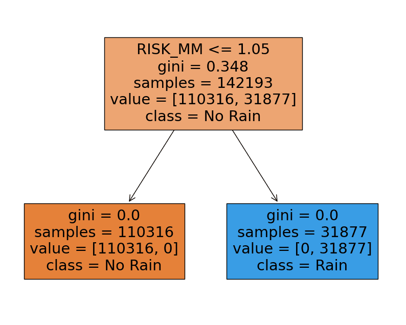
As you can see from the picture above, RISK_MM plays the most important role to decide wether its rain or not tomorrow.

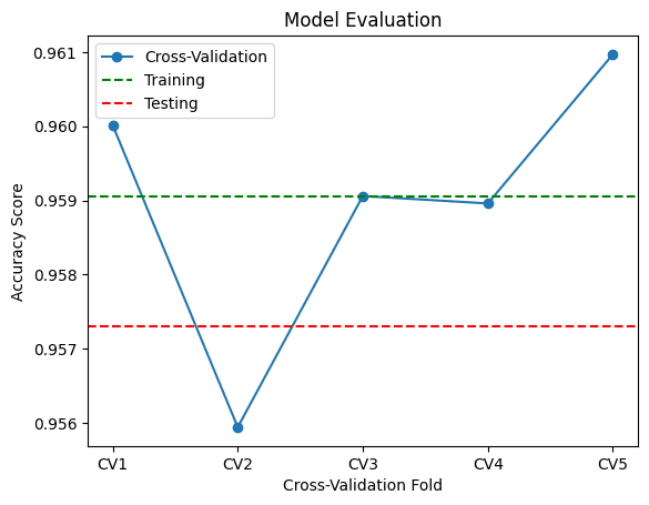
Now in case you need to see the Cross-Validation score, we will try to apply cross validation on gaussian model

from sklearn.model_selection import cross_val_score

model_gaussian = GaussianNB()
model_gaussian.fit(X, y)

cv_scores = cross_val_score(model_gaussian, X_train, y_train, cv=5, scoring='accuracy')

mean_score = cv_scores.mean()
std_score = cv_scores.std()

model_gaussian.fit(X_train, y_train)

train_score = model_gaussian.score(X_train, y_train)

test_score = model_gaussian.score(X_test, y_test)

print("Mean Cross-Validation Score:", mean_score)
print("Standard Deviation of Cross-Validation Scores:", std_score)
print("Training Score:", train_score)
print("Testing Score:", test_score)

Visualization

import matplotlib.pyplot as plt

# Plotting the scores
labels = ['CV1', 'CV2', 'CV3', 'CV4', 'CV5']
x = range(1, len(cv_scores) + 1)

plt.plot(x, cv_scores, marker='o', linestyle='-', label='Cross-Validation')
plt.axhline(y=train_score, color='green', linestyle='--', label='Training')
plt.axhline(y=test_score, color='red', linestyle='--', label='Testing')

plt.xlabel('Cross-Validation Fold')
plt.ylabel('Accuracy Score')
plt.title('Model Evaluation')
plt.xticks(x, labels)
plt.legend()
plt.show()

Decision Tree Structure

Read this

If you read this message, thanks for reading all the article. I just want to let you know that if u have any question, you can email me at shizuka0@proton.me

Also i made a paper about this, not official though, in case you need it just ask in the email, the paper is in Indonesia language.

Thanks! Love u ❤️

References