Perceptron with Iris Dataset

A perceptron is a basic linear classifier used in machine learning. It takes input features, applies weights and a bias term, computes a sum, and passes it through an activation function to produce an output. The perceptron adjusts its weights and bias during training based on classification errors. It is limited to learning linearly separable patterns. This time, we will try to apply perceptron algorithm using iris dataset.

Before we jump into preprocessing, training and testing, we need to make some perceptron function first.

1. Step Perceptronn

def percep_step(input, th=0):
  return 1 if input > th else -1 if input < -th else 0

2. Training Perceptron

def percep_fit(X, target, th=0, a=0.01, max_epoch=-1, verbose=False,draw=False):
  w = np.zeros(len(X[0]) + 1)
  bias = np.ones((len(X), 1))
  X = np.hstack((bias, X))
  stop = False
  epoch = 0

  while not stop and (max_epoch == -1 or epoch < max_epoch):
      stop = True
      epoch += 1

      if verbose:
        print('\nEpoch', epoch)

      for r, row in enumerate(X):
        y_in = np.dot(row, w)
        y = percep_step(y_in, th)

        if y != target[r]:
          stop = False
          w = [w[i] + a * target[r] * row[i] for i in range(len(row))]
        if verbose:
          print('Weight:', w)
        if draw:
          plot(line(w, th), line(w, -th), X, target)

  return w, epoch

3. Testing Perceptron

def percep_predict(X, w, th=0):
  Y = []
  for x in X:
    y_in = w[0] + np.dot(x, w[1:])
    y = percep_step(y_in, th)
    Y.append(y)
  return Y

4. Calculate Accuracy

def calc_accuracy(a, b):
  s = [1 if a[i] == b[i] else 0 for i in range(len(a))]
  return sum(s) / len(a)

5. Plotting Function

import matplotlib.pyplot as plt
import numpy as np

def line(w, th=0):
    w2 = w[2] + .001 if w[2] == 0 else w[2]

    return lambda x: (th - w[1] * x - w[0]) / w2


def plot(f1, f2, X, target, padding=1, marker='o'):
    X = np.array(X)

    x_vals, y_vals = X[:, 1], X[:, 2]
    xmin, xmax, ymin, ymax = x_vals.min(), x_vals.max(), y_vals.min(), y_vals.max()
    markers = f'r{marker}', f'b{marker}'
    line_x = np.arange(xmin-padding-1, xmax+padding+1)

    for c, v in enumerate(np.unique(target)):
        p = X[np.where(target == v)]

        plt.plot(p[:,1], p[:,2], markers[c])

    plt.axis([xmin-padding, xmax+padding, ymin-padding, ymax+padding])
    plt.plot(line_x, f1(line_x))
    plt.plot(line_x, f2(line_x))
    plt.show()

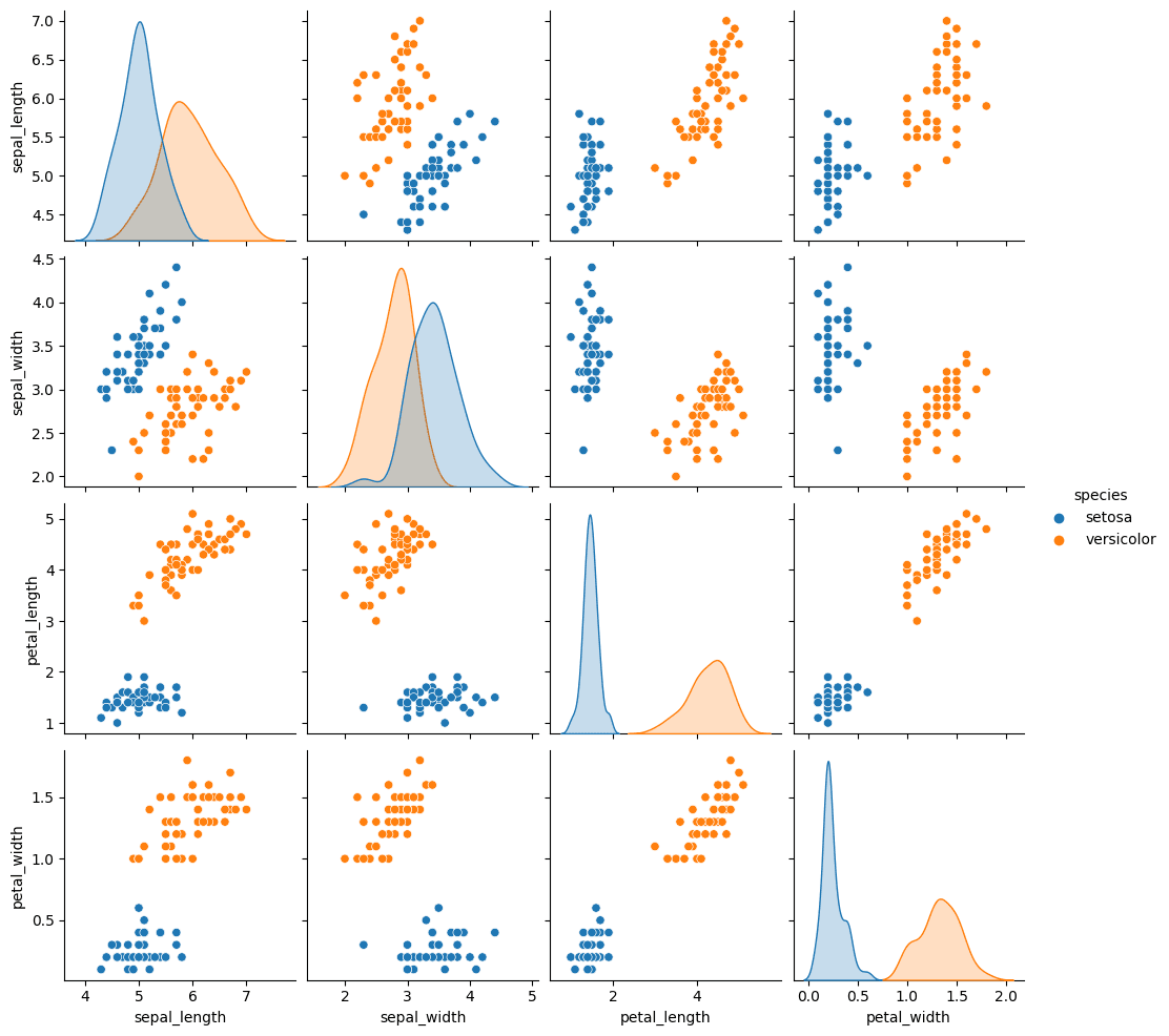
After the preparation, we finally can to start to process the dataset. First, need to load iris dataset.

import seaborn as sns
import matplotlib.pyplot as plt

iris = sns.load_dataset('iris')

sns.pairplot(iris, hue='species')
plt.show()

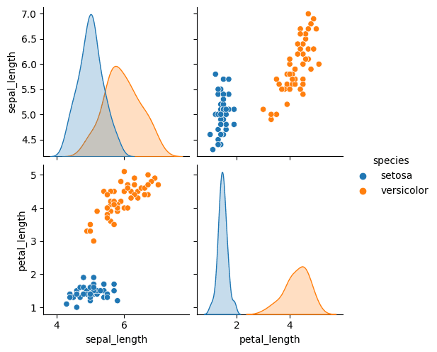
Because perceptron only has Bipolar target (the target can only 1 or -1), then we need to drop other column and leaving 2 column. In this case, we will delete Virginica.

iris = iris.loc[iris['species'] != 'virginica']

sns.pairplot(iris, hue='species')
plt.show()

Distribution of the sentosa and versicolor classes

As mentioned above, that perceptron target is only bipolar. But this case is only applied to target/classes. You can have as many features as you want. But in this case, we will delete sepal_width and petal_width.

iris = iris.drop(['sepal_width', 'petal_width'], axis=1)

sns.pairplot(iris, hue='species')
plt.show()

CSS greatly affects page load time

As you can see from the picture above, the two classes are perfectly separated. This is good sign since its for practice purpose only. The next thing we will do is testing and training.

from sklearn.model_selection import train_test_split
from sklearn.preprocessing import minmax_scale

X = iris[['sepal_length', 'petal_length', 'sepal_width','petal_width']].to_numpy()
X = minmax_scale(X)

y = iris['species'].to_numpy()
c = {'setosa': -1, 'versicolor': 1}
y = [c[i] for i in y]

X_train, X_test, y_train, y_test = train_test_split(X, y, test_size=.3)
w, epoch = percep_fit(X_train, y_train, verbose=True, draw=True)
out = percep_predict(X_test, w)
accuracy = calc_accuracy(out, y_test)

print('Epochs:', epoch)
print('Accuracy:', accuracy)

Final train with accuracy 1

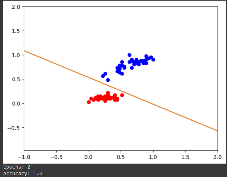
From the image above, we can see that our model can accurately predict the classes of iris. This is proven by looking at the line in the picture above. The line is called decision boundaries. The reason we have 100% accuracy is because the line manages to separate the red and blue dots perfectly

References

Implementing Perceptron with Python

Happy DLearn-ing!