Why Filling Null Values with the Mean Is Such a Bad Idea

Missing data is a common problem in real-world datasets across many domains. Imputation techniques are used to replace missing values with plausible substitutes to enable analysis on complete datasets. Two popular imputation approaches are Mean Imputer and Multivariate Imputation by Chained Equations (MICE).

Mean Imputer is a simple technique that replaces missing values with the mean/median of the available cases for that feature. While easy to implement, it makes the strong assumption that missing values are missing completely at random.

MICE is an advanced model-based technique that draws imputations from a sequence of conditional models, where each imputed variable is modeled conditional upon others in the data. This allows MICE to capture relationships among variables when imputing.

In this experiment we will use the infamous iris dataset and try to compare the performance of both imputer. So, let's jump in!

1. Import Libraries

from sklearn.datasets import load_iris
import matplotlib.pyplot as plt
import seaborn as sns
import pandas as pd
import numpy as np
from sklearn.experimental import enable_iterative_imputer
from sklearn.impute import IterativeImputer
from sklearn.metrics import mean_squared_error
from sklearn.model_selection import train_test_split
from sklearn.neighbors import KNeighborsClassifier
from sklearn.metrics import accuracy_score

2. Load Dataset

iris = load_iris()
data = pd.DataFrame(data=np.c_[iris['data'], iris['target']], columns=iris['feature_names'] + ['target'])
data = data.drop(['petal length (cm)','petal width (cm)'], axis=1)

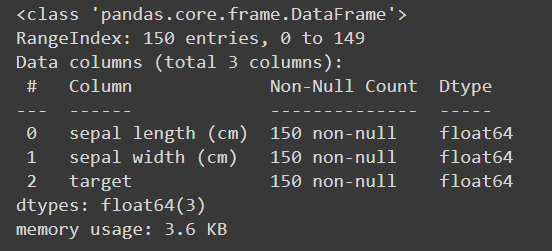
data.info()
feature = 'sepal length (cm)'

We will use iris dataset that is provided by sklearn. For this experiment we will delete petal features from the dataset. Why? this will helps us to compare the training result later. More data = more accurate the model is hence we won't be able to see the difference. We will also make sepal length as variabel to compare here.

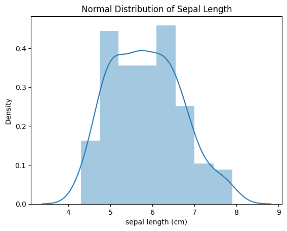
3. Visualize Normal Distribution

4. Filling with Mean

# Copy DataFrame and remove randomly 50 values in 'sepal length (cm)' column to null
data_knn = data.copy()
indices = np.random.choice(data_knn.index, 50, replace=False)
original_values = data_knn.loc[indices, feature].copy()
data_knn.loc[indices, feature] = np.nan

# Fill the null values with mean
mean_width = data_knn[feature].mean()
data_knn[feature].fillna(mean_width, inplace=True)

# Visualize the normal distribution after filling null values
sns.distplot(data_knn[feature], kde=True)
plt.title('Normal Distribution of Sepal Length (Filling Null With Mean)')
plt.show()

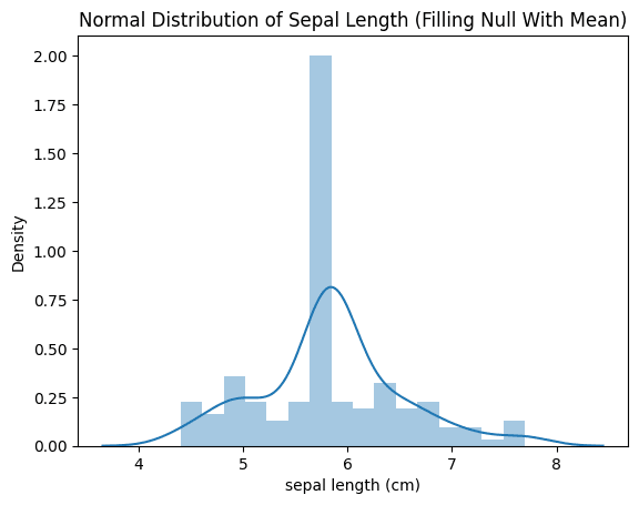
From the picture above we can tell that the distribution of imputed values did not match the original distribution of the non-missing data. Mean Imputer tends to make the data distributions narrower and less variable.

What do you mean by less variable? this means that the process of imputing missing values using the mean value of the available data tends to reduce the range and variability of the imputed values compared to the original non-missing data.

4. Filling with MICE

# Copy DataFrame and remove randomly 50 values in 'sepal length (cm)' column to null
data_mice = data.copy()
data_mice.loc[indices, feature] = np.nan

# Fill the null values with mice
imputer = IterativeImputer(random_state=42, max_iter=10, verbose=True)
imputer.fit(data_mice)
X_imputed = imputer.transform(data_mice)

# Visualize the normal distribution after filling null values
sns.distplot(data_mice[feature], kde=True)
plt.title('Normal Distribution of Sepal Length (Filling Null With MICE)')
plt.show()

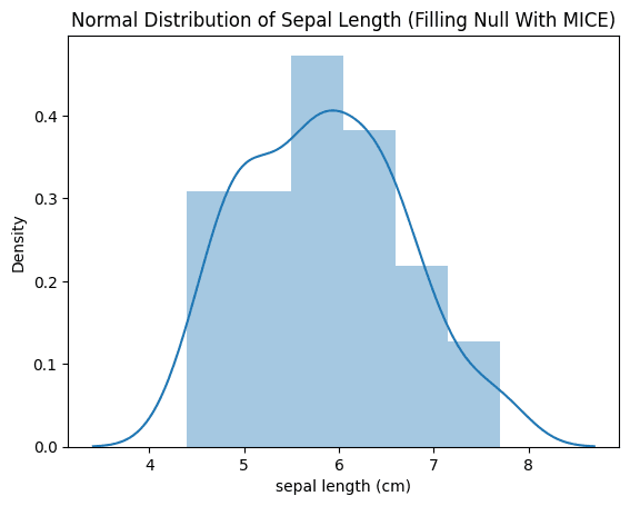
From the picture above the MICE (Multiple Imputation by Chained Equations) method successfully maintained the original distribution of the data across all the variables in the dataset with less loss.

How is this possible though? MICE utilizes the relationships between variables during its step-by-step imputation procedure, which helps to preserve valuable structural information within the data.

5. Compare Loss Values

imputed_values = data_knn.loc[indices, feature]
loss = mean_squared_error(original_values, imputed_values)
print(f"Mean Squared Error (Loss) between original and imputed Mean: {loss}")

#convert mice imputed numpy array to dataframe
data_mice = pd.DataFrame(X_imputed, columns=['sepal length (cm)', 'sepal width (cm)', 'target'])

imputed_values = data_mice.loc[indices, feature]
loss = mean_squared_error(original_values, imputed_values)
print(f"Mean Squared Error (Loss) between original and imputed MICE: {loss}")

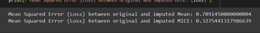
Based on the provided image we can see that the mean squared error was around 0.4 higher for Mean Imputer compared to MICE. This shows that MICE produces more accurate imputations by effectively utilizing the relationships and patterns found in the available portions of the data.

6. Compare Training Accuracy

For training we will use the infamous machine learning method, which is K-Nearest Neighbor (KNN).

Mean Imputed Training

X = data_knn.drop('target', axis=1)
y = data_knn['target']

X_train, X_test, y_train, y_test = train_test_split(X, y, test_size=0.3, random_state=42)

model = KNeighborsClassifier()
model.fit(X_train, y_train)
y_pred = model.predict(X_test)
accuracy = accuracy_score(y_test, y_pred)
print(f"{type(model).__name__} Accuracy: {accuracy:.2f}")

MICE Imputed Training

X = data_mice.drop('target', axis=1)
y = data_mice['target']

X_train, X_test, y_train, y_test = train_test_split(X, y, test_size=0.3, random_state=42)

model = KNeighborsClassifier()
model.fit(X_train, y_train)
y_pred = model.predict(X_test)
accuracy = accuracy_score(y_test, y_pred)
print(f"{type(model).__name__} Accuracy: {accuracy:.2f}")

As shown in the picture, it is clear that with the Mean Imputed data, the classification accuracy was only 0.78. In contrast, with the MICE imputed data, the accuracy jumped to an impressive 0.93.

That accuracy results highlight how better imputation techniques like MICE do not just restore missing values more accurately, but can also significantly boost performance on actual analytical tasks and models built on the imputed data.

7. Conclusion

The findings show that using advanced methods like MICE to fill in missing data is better than simpler methods like Mean Imputation, especially when:

• It's important to keep the original patterns of the data intact.
• The variables are connected to each other in some way that can be used.
• The filled-in data will be used in other analysis models later on.

The Mean Imputer method is simple but it makes assumptions that can change the characteristics of the data. Advanced techniques like MICE are better at dealing with missing data in a more detailed way without losing the accuracy of the original dataset. This experiment demonstrates that,

Putting more effort into improving the way we fill in missing data can result in significant benefits.

Thanks for reading ! 🥰😼🤟

References

• MICE Documentation on Sklearn
• K-Nearest Neighbors Documentation on Sklearn
• Understanding How MICE Works Under the Hood

Happy DLearn-ing!